Cloud-Optimized Geotiff methods for GEFS
gefs-cog.RmdIn this vignette we take a look at assembling on-demand data cubes from the NOAA Global Ensemble Forecast System which can be used as driver data for forecasts anywhere in the world.
knitr::opts_chunk$set(message=FALSE, warning=FALSE, fig.path = "man/figures/")In addition to this package (gefs4cast), this approach
relies heavily on the amazing and innovative work of
gdalcubes, as well as few commonly used packages.
library(gdalcubes)
library(gefs4cast) # remotes::install_github("neon4cast/gefs4cast")
library(stringr)
library(lubridate)
library(stars)
library(viridisLite)
library(tmap)

gdalcubes_options(parallel = 24)
Accessing GEFS data
First, we use gefs4cast to download the GEFS average
forecast for the next 10 days. While it is possible to download each of
the ensemble members individually, and also possible to access forecasts
up to 35 days in advance, this gives a nice dataset for experimentation
and illustrative purposes.
The raw data consists of one file every for every 3 hours over the 240 hour (10 day) forecast horizon, some 80 GRIB files in total, hosted freely accessible on Amazon Web Services. Each file contains global coverage for some 80 bands, of which we access the ground-height (2m or 10m) values for seven common variables.
In an idealized workflow, these files would be avialable in a
Cloud-optimized format like GeoTIFF and indexed in a STAC Catalog.
Meanwhile, gefs4cast takes on the responsibility of rapidly
downloading the desired bands while converting these GRIB files to local
GeoTIFF files using command-line gdaltranslate utilities in
parallel. This is quite fast, especially if significant bandwidth and
processing power are available, but reasonably crude.
date <- as.Date("2022-12-05") #Sys.Date()
gefsdir <- tempfile()
## 3-hr period up to 10 days, (then every 6 hrs up to 35 day horizon)
gefs_cog(gefsdir, ens_avg=TRUE,
         max_horizon=240, date = date) |>
  system.time()
## user system elapsed
## 101.574 13.401 9.399Constructing a data cube
With our 80 files in hand, it is time to assemble them into a multi-band “data cube”. We specify the datetimes by parsing the horizon notation from the filename and the bands from the encoded file metadata.
Given the band names and date range, we can use
gdalcubes to construct an image collection of all 79 assets
(note the horizon=0 file uses an incompatible band structure and is
omitted here).
# 000 file has different bands and so cannot be stacked into the collection
files <- fs::dir_ls(gefsdir, type="file", recurse = TRUE)[-1]
step <- files |> str_extract("f\\d{3}\\.tif") |> str_extract("\\d{3}")
datetime <- Sys.Date() + hours(step)

# pull band names out with stars, hack the timestamp off of the band name
fc <- stars::read_stars(files[1])
bandnames <-
  stars::st_get_dimension_values(fc, 3) |>
  stringr::str_extract("([A-Z]+):") |> str_remove(":")

gefs_cube <- create_image_collection(files,
                                     date_time = datetime,
                                     band_names = bandnames)
Constructing a cube view
Second, we can create an entirely abstract “cube view” representing
our desired spatial and temporal resolution. For the moment, we simply
use the full time and space range of the assets, as well as the original
0.5 degree spatial resolution dx,dy and 3 hour
temporal resolution (dt = "PT3H", in ISO Period
notation).
A crucial observation here, as we shall soon see, is that we are by no means obligated to stick with either the projection, the spatial/temporal extent or resolution of the data itself – we can ask for whatever we want in defining this abstract box!
box <- sf::st_bbox(fc)
iso <-"%Y-%m-%dT%H:%M:%S"
ext <- list(t0 = as.character(min(datetime),iso),
              t1 = as.character(max(datetime),iso),
              left = box[1], right = box[3],
              top = box[4], bottom = box[2])
v <- cube_view(srs = "EPSG:4326",
               extent = ext,
              dx = 0.5, dy = 0.5, # original resolution -- half-degree
              dt = "PT3H",   # original resolution
               aggregation = "mean", resampling = "cubicspline"
)
It is worth thinking about each of these elements for a moment
Projection. This one is perhaps most obvious. Specifying the projection is not only a way to define the units which our box boundaries are specified in, our data will also be transformed automatically into whatever projection we select. This is much better than typical manual tooling that expects us to re-project. Projections can be given as EPSG codes or full WKT strings.
Extent We are free to set an extent in space or time that is larger or smaller than our data. Intuitively, setting a smaller range in space or time allows us to subset our original collection in that way. Setting a larger spatial or temporal extent than the data covers will introduce missing values.
Resolution Resolution is perhaps the least obvious and most magical.
First, we could choose to set a resolution in space, that is coarser than the underlying data, e.g.dx=1.0anddy=1.0. In such cases, the data will be automatically coarse-grained for us. This can be especially useful when generating large-spatial scale analyses from fine-scale data (e.g. continental scale analyses from high resolution imagery like Sentinel-2). Perhaps more remarkably, we can also request a resolution that is finer than the data itself: e.g.dx=0.25, dy=0.25, or even finer. In these cases, the data products will be automatically re-sampled to interpolate finer-scale pixel values (usinggdalwarpunder the hood). A variety of resampling algorithms are possible, from simplest (nearest neighbor) to richer methods like cubic splines. Theresamplingargument specifies the algorithm for how pixels are resampled across space to achieve the desired resolution.Temporal Resolution: Just as we can set resolution in space, we can also choose a resolution in time. Here, we have specified a the 3-hour interval, matching the data. If we specify a coarser interval, multiple images covering the same pixels during that interval will be aggregated. If we specify a finer time interval than the data, the intermediate intervals are not automatically filled in by algorithm, but are treated as missing data. We can later fill these in through interpolation using the
fill_time()method.
With GEFS, each single asset file represents spatial coverage of the
whole globe, and no pixels are obscured by clouds or otherwise missing
measurements. With other remote sensing products, our collection may
consist of a mosaic of interlocking or even overlapping tiles. Such
mosiacs work equally well, with an optional mask argument
allowing bad pixels such as cloud cover to be removed, and then
automatically filled in by the aggregation method from any overlapping
images within the specified time interval.
Applying our cube view to the GEFS data
Let’s take a look at the temperature data cube now. Animations
provide a natural way to visualize spatio-temporal data, and are easy to
produce. All gdalcubes calculations are lazy-evaluated, so
that calculations are done only when necessary and only at the
resolution required for the operation. Crucially, calculations are also
entirely streaming, and thus require very little RAM despite the often
masssive scale of the data sets involved.
raster_cube(gefs_cube, v) |>
  gdalcubes::select_bands("TMP") |>
  animate( col = viridisLite::viridis, nbreaks=100,
           fps=10, save_as = "temp.gif")
Because the cube_view specification is completely
abstract and distinct from the data assets, we can
easily define a desired cube view that we reuse across a wide variety of
data sources – from GEFS to MODIS to Sentinel etc, extracting data in
identical spatio-temporal extents and resolutions.
The necessary CRS transforms, cropping, coarse-graining or downscaling,
averaging or interpolating is all baked into the abstraction and handled
in parallelized and high-performance operations behind the scenes.
Downward Shortwave Radiation Flux is a good way to see what parts of the globe are in day and night:
raster_cube(gefs_cube, v) |>
  gdalcubes::select_bands("DSWRF") |>
  animate( col = viridisLite::viridis, nbreaks=100,
           fps=2, save_as = "dswrf.gif")
## [1] "/home/cboettig/eco4cast/gefs4cast/vignettes/dswrf.gif"
Downscaling to finer resolution
GEFS predictions are relatively coarse in space. For EFI terrestrial forecast, finer temporal scales may also be desirable, such as for driving the 30min terrestrial forecast. Let us thus consider a finer spatial and temporal scale in our view. Further, we need not consider the full global extent of the data. For illustrative purposes, lets focus on a much smaller but still considerable spatial scale of the northeastern US. We define two views of this area, one at the original resolution and the other at finer spatial resolution. (While it is possible to use a finer temporal resolution as well, as shown, this is not necessary – temporal interpolation does not happen automatically, and we can perform this step on the fly later on.)
box <- c(-75, 40, -70, 44)
ext <- list(t0 = as.character(min(datetime),iso),
             t1 = as.character(max(datetime),iso),
             left = box[1], right = box[3],
             top = box[4], bottom = box[2])

v_orig <- cube_view(srs = "EPSG:4326",
                    extent = ext,
                    dx = 0.5, dy = 0.5,
                    dt = "PT3H",
                    aggregation = "mean",
                    resampling = "cubicspline"
    )

v_fine <- cube_view(srs = "EPSG:4326",
                    extent = ext,
                    dx = 0.1, dy = 0.1,
                    dt = "PT30M",
                    aggregation = "mean",
                    resampling = "cubicspline"
    )
For reference, let’s first see what the raw data looks like at this level:
t <- as.character(datetime[[3]], iso)
t
## [1] "2022-12-09T09:00:00"
raster_cube(gefs_cube, v_orig) |>
   gdalcubes::select_bands("TMP") |>
   slice_time(datetime = t) |>
   st_as_stars() |>
   tm_shape() + tm_raster(palette=viridis(100), n = 100,
                          legend.show=FALSE, style = "cont") +
   tm_shape(spData::us_states) + tm_polygons(alpha=0, border.col = "grey")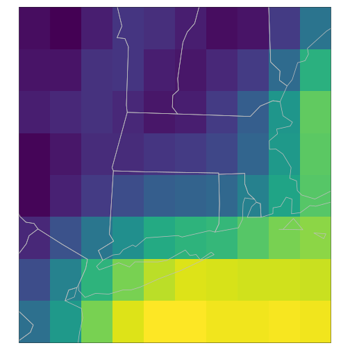
plot of chunk tmap_orig
Temporal interpolation
raster_cube(gefs_cube, v_fine) |>
   gdalcubes::select_bands("TMP") |>
   slice_time(datetime = t) |>
   st_as_stars() |>
   tm_shape() + tm_raster(palette=viridis(100), n = 100,
                          legend.show=FALSE, style = "cont") +
   tm_shape(spData::us_states) + tm_polygons(alpha=0, border.col = "grey")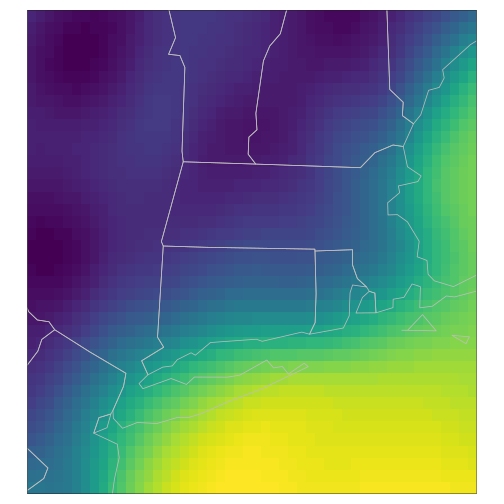
plot of chunk tmap_fine
Temporal interpolation is not performed by default, but we can
interpolate data to an arbitrarily finer timescale. (Note that if we did
not fill_time(), the result would be all-missing temp data.
Meanwhile, also note we can ask for an arbitrarily fine time scale here,
and do so on the v_orig data as well.)
# an intermediate time:
t2 <- as.character(as_datetime(t) + minutes(30),  iso)
t2
## [1] "2022-12-09T09:30:00"
raster_cube(gefs_cube, v_fine) |>
   gdalcubes::select_bands("TMP") |>
   gdalcubes::fill_time("linear") |>
   slice_time(datetime = t2) |>
   st_as_stars() |>
   tm_shape() + tm_raster(palette=viridis(100), n = 100,
                          legend.show=FALSE, style = "cont") +
   tm_shape(spData::us_states) + tm_polygons(alpha=0, border.col = "grey")
Extracting values
As illustrated in these examples, any data cube can be coerced into a
stars object, and we can use all the classic manipulation techniques
available in stars, e.g. to extract values at particular set of spatial
points over all time. We then use classic tidyverse to pivot the
resulting array into a simple data.frame of site_id,
datetime, predicted, and variable
for the chosen reference datetime here.
sites <- neon_coordinates() |>
  tibble::as_tibble(rownames = "site_id") |>
  sf::st_as_sf(coords= c("longitude", "latitude"), crs="EPSG:4326")

df <- raster_cube(gefs_cube, v) |> extract_geom(sites)
extract_geom() returns a data.frame with columns for
time, feature ID (FID, i.e. row-number matching the polygon
for the site), and columns for each band. We can easily pivot this into
Ecological Forecasting Initiative (EFI) format.
library(tidyverse)
fc <- sites |>
  tibble::rowid_to_column(var="FID") |>
  inner_join(df) |>
  as_tibble() |>
  select(-FID, -geometry) |>
  pivot_longer(c(-time, -site_id),
               names_to="variable",
               values_to="prediction")

head(fc)
## # A tibble: 6 × 4
## site_id time variable prediction
## <chr> <chr> <chr> <dbl>
## 1 LIRO 2022-12-10T15:00:00 APCP 0
## 2 LIRO 2022-12-10T15:00:00 DLWRF 185.
## 3 LIRO 2022-12-10T15:00:00 DSWRF 37.2
## 4 LIRO 2022-12-10T15:00:00 PRES 96120.
## 5 LIRO 2022-12-10T15:00:00 RH 76.3
## 6 LIRO 2022-12-10T15:00:00 TMP -10.1Working directly with the gdalcube however, we can already also
perform much richer calculations with reduce_time,
reduce_space, pixel_apply,
chunk_apply and other functions of the gdalcubes
packages.