Example of interacting with and visualizing EFI standard data
visualization-example.Rmd
library(EML)
library(emld)
library(lubridate)
library(tibble)
library(dplyr)
library(tidyr)
library(ggplot2)
library(EFIstandards)
Visualizing the simple, example forecast of population growth of two interacting species
========================================================
Parsing metadata
First load the data using EML.
eml_filename <- system.file("extdata", "forecast-eml.xml", package="EFIstandards")
md <- read_eml(eml_filename)  #you could replace the variable here with a filename form a downloaded data package from a repository
Then to examine the details, use EML::eml_get. First,
the title and abstract and who made it.
eml_get(md, "title")## '': A very simple Lotka-Volterra forecast
eml_get(md, "abstract")## '': An illustration of how we might use EML metadata to describe an ecological forecast
eml_get(md, "creator")## electronicMailAddress: rqthomas@vt.edu
## id: https://orcid.org/0000-0003-1282-7825
## individualName:
## givenName: Quinn
## surName: ThomasThen diving in, the coverage and keywords
eml_get(md, "coverage")## geographicCoverage:
## geographicDescription: 'Lake Sunapee, NH, USA '
## boundingCoordinates:
## westBoundingCoordinate: '-72.15'
## eastBoundingCoordinate: '-72.05'
## northBoundingCoordinate: '43.48'
## southBoundingCoordinate: '43.36'
## taxonomicCoverage:
## taxonomicClassification:
## - taxonRankName: Genus
## taxonRankValue: Gloeotrichia
## taxonomicClassification:
## taxonRankName: Species
## taxonRankValue: echinulata
## - taxonRankName: Genus
## taxonRankValue: Anabaena
## taxonomicClassification:
## taxonRankName: Species
## taxonRankValue: circinalis
## temporalCoverage:
## rangeOfDates:
## beginDate:
## calendarDate: '2001-03-04'
## endDate:
## calendarDate: '2001-04-02'
eml_get(md, "keywordSet")## keyword:
## - forecast
## - population
## - timeseries
## keywordThesaurus: EFI controlled vocabularyLooks like it’s a population level timeseries forecast of Lake Sunapee, NH, USA for two species:
# these seem a bit of a pain to pull out maybe there's an easier way
spps <- eml_get(md, "taxonRankValue")
sp1 <- paste(spps[1:2], collapse=" ")
sp2 <- paste(spps[3:4], collapse=" ")
sp1
## [1] "Gloeotrichia echinulata"
sp2## [1] "Anabaena circinalis"Reading structured methods
Load the additional metadata (see documentation of EFI forecasting standard):
methods_md <- eml_get(md, "additionalMetadata")
methods_md
## metadata:
## forecast:
## drivers:
## status: absent
## forecast_horizon: 30 days
## forecast_issue_time: '2001-03-04'
## forecast_iteration_id: 20010304T060000
## forecast_project_id: LogisticDemo
## initial_conditions:
## complexity: '2'
## status: present
## metadata_standard_version: '0.3'
## model_description:
## forecast_model_id: v0.3
## name: discrete Lotka–Volterra model
## repository: https://github.com/eco4cast/EFIstandards/blob/master/vignettes/logistic-metadata-example.Rmd
## type: process-based
## obs_error:
## complexity: '2'
## covariance: 'FALSE'
## status: present
## parameters:
## complexity: '6'
## status: present
## process_error:
## complexity: '2'
## covariance: 'FALSE'
## propagation:
##   size: '10'
##   type: ensemble
## status: propagates
## random_effects:
## status: absent
## timestep: 1 dayThis metadata contains details about the system forecast including number of state variables and parameters, and the methods used, including propagation of uncertainty. For example, details of the treatment of process error in this model are given by
## complexity: '2'
## covariance: 'FALSE'
## propagation:
## size: '10'
## type: ensemble
## status: propagates
n_ensembles <- methods_md %>% eml_get("process_error") %>% eml_get("size")
n_ensembles <- n_ensembles[[1]]
From this metadata, the output of this forecast should have error propagation via an ensemble of size 10, process error for two state varible dimensions with no covariance between these. Further, one can check if the forecast used data assimilation (no):
eml_get(md, "assimilation")## {}Output metadata
Finally, I’ll dive into the metadata for the output data itself. Wait, which output data? All we’ve seen so far is metadata!
First remember that EML specifies a tag “physical” for the location of an actual data file. There’s plenty of metadata on the file itself including authentication format, etc
## authentication:
##   method: MD5
##   authentication: 4dbe687fa1f5fc0ff789096076eebd78
## dataFormat:
##   textFormat:
##     recordDelimiter: |2+
##
##     attributeOrientation: column
##     simpleDelimited:
##       fieldDelimiter: ','
## objectName: logistic-forecast-ensemble-multi-variable-multi-depth.csv
## size:
##   unit: bytes
##   size: '110780'
To get the data parse the filename and load it!
datafilename <- eml_get(dt_md, "objectName")[[1]]
# this steps are necessary because this is in an R package if you have a downloaded data repository
# you coudl just pass 'datafilename' into read.csv here
datafile <- system.file("extdata", datafilename, package="EFIstandards")
dt <- as_tibble(read.csv(datafile, row.names=1))
dt
## # A tibble: 1,800 × 8
## time depth ensemble obs_flag species_1 species_2 forecast data_assimilati…
## <chr> <int> <int> <int> <dbl> <dbl> <int> <int>
## 1 2001-0… 1 1 1 0.5 0.5 0 0
## 2 2001-0… 3 1 1 0.5 0.5 0 0
## 3 2001-0… 5 1 1 0.5 0.5 0 0
## 4 2001-0… 1 2 1 0.5 0.5 0 0
## 5 2001-0… 3 2 1 0.5 0.5 0 0
## 6 2001-0… 5 2 1 0.5 0.5 0 0
## 7 2001-0… 1 3 1 0.5 0.5 0 0
## 8 2001-0… 3 3 1 0.5 0.5 0 0
## 9 2001-0… 5 3 1 0.5 0.5 0 0
## 10 2001-0… 1 4 1 0.5 0.5 0 0
## # … with 1,790 more rowsOK! This has the column names and actual data. To understand these
column names, recall the output dataset metadata, which was loaded
earlier. In particular the attributeList contains fine
details like units and definitions for each column:
dt_md_cols <- dt_md %>% eml_get("attributeList") %>% get_attributes()
dt_md_cols$attributes
## attributeName attributeDefinition storageType
## 1 time [dimension]{time} date
## 2 depth [dimension]{depth in reservior} float
## 3 ensemble [dimension]{index of ensemble member} float
## 4 obs_flag [dimension]{observation error} float
## 5 species_1 [variable]{Pop. density of species 1} float
## 6 species_2 [variable]{Pop. density of species 2} float
## 7 forecast [flag]{whether time step assimilated data} float
## 8 data_assimilation [flag]{whether time step assimilated data} float
## formatString measurementScale domain unit numberType
## 1 YYYY-MM-DD dateTime dateTimeDomain <NA> <NA>
## 2 <NA> ratio numericDomain meter real
## 3 <NA> ratio numericDomain dimensionless integer
## 4 <NA> ratio numericDomain dimensionless integer
## 5 <NA> ratio numericDomain numberPerMeterSquared real
## 6 <NA> ratio numericDomain numberPerMeterSquared real
## 7 <NA> ratio numericDomain dimensionless integer
## 8 <NA> ratio numericDomain dimensionless integerCross-referencing this documentation of EFI forecasting standards,
note that data_assimilation column is zeroed out so this
performed no data assimilation and forecast column is
zeroed out so this was a hindcast. As expected, there are 10 ensemble
members in the forecast. As consumer of this type of forecast this is
the only way to understand the uncertainty in the forecast.
Visualizing the data
The output includes densities (number per meter squared) for both
species 1 and species 2. I assume these are in the same order as the
entries in taxononmicCoverage: Gloeotrichia echinulata and
Anabaena circinalis at several depths measured in meters. Glancing at
column depth there are only three depths represented. While
reshaping the data, I will rename columns with useful information about
their units and construct a categorical variable with the actual species
names:
dtl <- pivot_longer(dt, c("species_1", "species_2"), values_to="density (m^-2)") %>%
  mutate(time = as.POSIXct(time),
         name=recode(name, species_1=sp1, species_2=sp2),
         `depth (m)` = depth)
Given the ensembles, order statitics or quantiles seem like a natural choice to summarize uncertainty, so compute the median and upper and lower quartiles:
dtl <- dtl %>%
  group_by(name, depth, time) %>%
  mutate(density_50 = median(`density (m^-2)`),
         density_25 = quantile(`density (m^-2)`, .25),
         density_75 = quantile(`density (m^-2)`, .75)
         )
Putting these pieces together to visualize and describe the forecast and its uncertainty:
ggplot(dtl) +
  geom_ribbon(aes(time, ymin=density_25, ymax=density_75, fill=name), alpha=0.3) +
  geom_line(aes(time, `density (m^-2)`, color=name, group=interaction(name, ensemble)), alpha=0.5) +
  #geom_smooth(aes(group=name), method='gam', formula= y ~ s(x, bs = "cs", k=30)) +
  geom_line(aes(time, density_50, color=name), size=1.25) +
  facet_grid(`depth (m)` ~ ., labeller=label_both) +
  guides(color=guide_legend(title='Median density'),
         fill=guide_legend(title='25th-75th quantile density')) +
  labs(title=eml_get(md, 'title')[[1]],
       subtitle=paste("Forecast from", n_ensembles, "ensembles (thin lines), with uncertainty from quantiles."),
       caption=paste("Demo visualization from EFIstandards package for an \nimaginary forecast at", eml_get(md, "geographicDescription")[[1]]))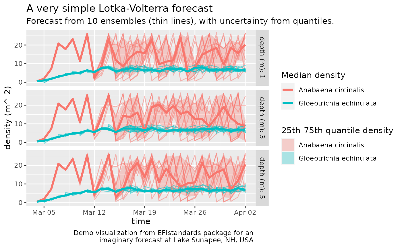
Forecast density of two interacting species at several depths with uncertainty.